
DNA Sequence Classification by CNN
Deep Learning Project. Dec 14, 2020
By Joely Nelson
In this project, I developed a convolutional neural network (CNN) to classify DNA sequences from two data sets. I mimic the architecture of the CNN used in prior work on two different datasets, and achieve close to the paper’s accuracy.
Intro
DNA carries genetic instructions for the development, function, growth and reproduction of all known organisms. DNA is essentially the programming language of life; information stored as A, T, G, and C. It makes sense that we should be able to use DNA sequences to make predictions about a gene’s function, classification, and transcription levels. However, this is extremely difficult, as there are many unknown features, and many bioinformatics algorithms must be generated by hand.
With the emergence of deep learning, which makes use of automatic feature learning, and the increase of available genetic data sets, there is an opportunity to apply deep learning to genetic datasets to make complex predictions. Machine learning models and deep neural networks have been used to predict the non-coding function of DNA, identifying DNA-binding proteins, and even predicting the transcription level of genes. This is still a new field and there is much more to be explored.
In this project, I tried to reproduce some of the work done in the paper DNA Sequence Classification by Convolutional Neural Network. Researchers treated DNA data like text and used CNNs to classify various DNA sequences. By reproducing their architecture, I am able to fine tune models that achieve close to their accuracy or better.
I wanted to do this project because I am currently applying data-driven approaches to learn more about the rules of CRISPR in the Carothers Research Group at the university of Washington. I am planning on implementing a network to classify and generate sequences that are good for CRISPR. I would like to better my understanding of making models with sequence data so when data for my project is collected, I’m ready to hit the ground running.
Data Processing
DNA sequences are represented as strings that typically contain only 4 different characters: A, T, G, and C. We can’t train our network with raw sequences. We will need to do some kind of preprocessing of our data before we can feed it into our neural network.
DNA as Text
In the paper I’m trying to mimic, researchers treated DNA sequences like text data, which gets converted into tokenized sequences before being fed into a neural network. Using this idea, we convert DNA sequences into tokenized sequences.
We require a dictionary that maps the various tokens in the sequence (ie ATCG) to a numerical token. Here is an example of a mapping from sequence letters to integer tokens:
{'A': 2, 'T': 3, 'C': 4, 'G':5}
Using this map we can convert DNA sequences into tokenized sequences. For example this sequence:
"GATCGTAGTCCTAGTAAGACTGAC"
Would be tokenized as this:
[5, 2, 3, 4, 5, 3, 2, 5, 3, 4, 4, 3, 2, 5, 3, 2, 2, 5, 2, 4, 3, 5, 2, 4]
Pad and Unknown Tokens
Although in the two datasets used for this project this problem is not encountered, it is possible the various input sequences in one dataset may be of different length. Unlike images or text, it may be unfeasible to resize or crop sequences. Instead we will add on an additional token, <pad> will go onto the tail end of any sequence that is too short.
It may also be possible that unknown tokens are found in that dataset, so we add on an <unk> token to represent unknown characters.
For example, if we had a dataset that consisted of the following two sequences:
'GATCGTAGTCCTAGTAAGACTGAC', 'TAGCC'
Then we might see a vocabulary to token mapping like this:
{'<pad>': 0, '<unk>': 1, 'A': 2, 'T': 3, 'C': 4, 'G': 5}
When tokenized and padded, the two sequences will look like this, respectively. Note the long train of 0s on the smaller sequence to represent the padding.
[5., 2., 3., 4., 5., 3., 2., 5., 3., 4., 4., 3., 2., 5., 3., 2., 2., 5., 2., 4., 3., 5., 2., 4.]
[3., 2., 5., 4., 4., 0., 0., 0., 0., 0., 0., 0., 0., 0., 0., 0., 0., 0., 0., 0., 0., 0., 0., 0.]
Architecture
I plan to mimic the architecture used in the paper. The description of their architecture is as follows:
“The model contains 2 convolutional layers. Each of these layers is followed by a subsampling layer. These layers are used to extract features from representation [matrices] of sequences. The extracted features are then transformed by using a fully connected neural network layer which contains 100 neurons. In this layer, we used a dropout value of 0.5 to reduce the effect overfitting. Finally, a soft max output layer is used to predict labels of input sequences.”
In my words, the tokenized input sequence is first put through an encoder. Then it goes through 2 layers that consist of a convolution, a RELU activation, and a max pool. The features are then flattened, and go through a fully connected layer that has an output of 100 features. A softmax is then applied, and the classification provided.
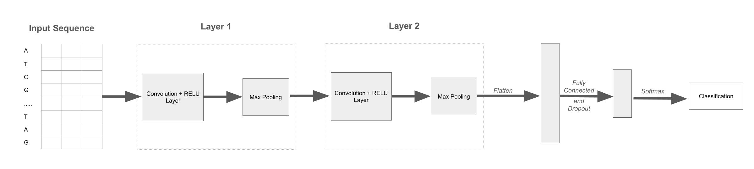
A visual representation of the network described
Although the paper recognizes the importance of hyperparameters, it does not provide any information about them (such as decay, learning rate, or momentum) nor kernel filters used in the convolutional layers. Trying to replicate the results by trying out different hyperparameters was the bulk of work for this project.
Although I played around with the hyperparameters extensively, I tried to keep the overall model architecture to what was specific to the best of my ability. The number of convolutional layers, the max pooling layer, the 100 neurons in the fully connected layer before the softmax, and the dropout value of 0.5, were kept the same for all experiments.
Their model has a 90% train 10% test split, and so the same will be used for this project. I also used cross entropy loss for all experiments.
Splice Dataset
Dataset can be downloaded here
This dataset contains information about splice junctions. In genes, regions which are removed during the RNA transcription process are called introns, and regions that are used to generate mRNA are called exons. Junctions between them are called splice junctions. There are two kinds of splice junction that is exon-intron junction, and intron-exon junctions.
Each of the sequences in this dataset are 60 base pairs long, and belong to one of 3 classes: “EI” (Extron-Intron junction), “IE” (Intron-Extron junction) and “N” (neither EI or IE). There are 767 genes with the EI label, 768 with the IE label, and 1655 with the N label.
The paper achieved a test accuracy of 96.18% for this dataset.
Model 1
The best model had a train accuracy of 99.33% (correctly classified 2852/2871 examples), and a test accuracy of 97.49% (correctly classified 311/319 examples).
The hyperparameters were as follows:
- feature_size = 60
- convolutional layer 1:
- kernel size: 6
- kernel stride: 3
- input channels: 60
- output channels: 480
- convolutional layer 2:
- kernel size: 6
- kernel stride: 3
- input channels: 240
- number of channels: 960
- decay = 0.01
- learning rate = 0.01
- momentum = 0.9
- epochs = 50
- pool type: 2d pool
I probably should have realized this sooner, but I realized that I was using a 2D pool instead of a 1D pool. I was unable to achieve the same level of accuracy, but got pretty close using a 1D pool and the same hyperparameters
The test accuracy was 1.31% better than the average accuracy reported in the paper. This implies that my model classifies 4 more examples in the test set correctly than the original paper.
Model 2
This second model uses all the same hyperparameters as the model above, but uses a 1D max pool and trains on less epochs than the previous one. This model had a train accuracy of 97.18% (correctly classified 2790/2871 examples), and a test accuracy of 97.18% (correctly classified 310/319 examples).
- feature_size = 60
- convolutional layer 1:
- kernel size: 6
- kernel stride: 3
- input channels: 60
- output channels: 480
- convolutional layer 2:
- kernel size: 6
- kernel stride: 3
- input channels: 240
- number of channels: 960
- decay = 0.01
- learning rate = 0.01
- momentum = 0.9
- epochs = 20
- pool type: 1d pool
This model does 1% better than the one from the paper, implying it classifies 1 more example correctly. This model correctly classifies 1 less example than the model that uses 2D pooling.
H3 Dataset
Dataset can be downloaded here
The H3 data set is of DNA sequences which wrap around histone proteins. It is a mechanism used to pack and store long DNA sequences into a cell’s nucleus. Sequences in this dataset are 500 base pairs long and belong to one of 2 classes: and belong to “Positive” or “Negative” class. Samples in “Positive” class contain regions wrapping around histone proteins. In contrast, samples in “Negative” class do not contain them. There are 7298 examples of the negative class, and 7667 examples of the positive class.
The paper was able to achieve an accuracy of 88.99% for this dataset. I was unable to achieve within less than 5% of this accuracy, here are the models that got closest.
Model 1
The best accuracy I achieved for the test set was 83.83% (correctly classified 1255/1497 examples), but this model had overfitting problems with a train accuracy of 91.12% (correctly classified 12273/13468 examples).
- feature_size = 500
- convolutional layer 1:
- kernel size: 12
- kernel stride: 6
- input channels: 500
- output channels: 1000
- convolutional layer 2:
- kernel size: 6
- kernel stride: 3
- input channels: 500
- output channels: 1000
- decay = 0.025
- learning rate = 0.001
- momentum = 0.9
- epochs = 25
- pool type: 2d pool
Model 2
Although this model didn’t achieve as good of a test accuracy as the model above, this one has less issues with overfitting. This had a test accuracy of 82.43% (correctly classified 1234/1497 examples), but this model had overfitting problems with a train accuracy of 85.87% (correctly classified 11565/13468 examples).
- feature_size = 2
- convolutional layer 1:
- kernel size: 6
- kernel stride: 3
- input channels: 2
- output channels: 10
- convolutional layer 2:
- kernel size: 6
- kernel stride: 3
- input channels: 50
- output channels: 400
- decay = 0.005
- learning rate = 0.001
- momentum = 0.9
- epochs = 50
- pool type: 2d pool
Discussion
The most important takeaway from this project for me was the importance of hyperparameters. Because the paper did not share the hyperparameters they chose, including the kernel size/stride of their convolutional layers, the learning rate, decay, and momentum, it was extremely difficult to replicate their results. Although I was able to beat the paper’s accuracy slightly for the splice dataset (~1%), I could not achieve the 88% accuracy for the H3 dataset, and instead was only able to get to 82%-83% test accuracy. If I had the paper’s hyperparameters, this would have been much more possible.
Another important note is that models that used 2D max pooling typically did better than models that used 1D max pooling. This may have been a fluke, but if this is a pattern this may be something that should be studied further.